German Railway Delay Analysis

Three stacked charts showing train count, average delay, and delay standard deviation by hour of day across 20 German stations

Peak hour analysis: train volume, average delay, and delay variability across 24 hours — evening cascading effects visible after 20:00

Solo project for the NoSQL/MongoDB course at HSLU. Nov 2025.

Overview

Deutsche Bahn operates one of Europe’s largest rail networks, and its delays are a constant topic in German public discourse. But most commentary is anecdotal — “trains are always late” — without data to show where delays accumulate, which stations manage them well, and when the network is under the most stress.

This project investigates those questions systematically. Using 6 days of real-time data from the DB OpenData API (14,743 scheduled trains, 52,005 real-time change records across 20 major stations), I built a complete ELT pipeline in Python and MongoDB and analyzed the network across multiple dimensions: station delay management efficiency, hub connectivity, train type specialization, corridor traffic patterns, and peak hour performance.

ELT Pipeline

Extract: Two parallel data streams — the Plan API returns scheduled timetables per station-hour (XML), while the Changes API captures real-time delays, cancellations, and platform changes. Custom XML parsers normalize both into structured Python dictionaries, filtering to long-distance services (ICE, IC, EC) and computing delay_minutes from planned vs. actual times.
Load: Raw documents stored in MongoDB Atlas across three collections (raw_timetable_plan, raw_timetable_changes, collection_log). A hierarchical collection architecture — single station-hour, daily, and multi-day campaign functions — enables both targeted extraction and automated batch processing.
Transform: A 10+ stage MongoDB aggregation pipeline merges plan and changes data via $lookup on journey_id, creating a unified journeys collection with computed fields (delay_change, is_peak_hour, station_improved_delay).

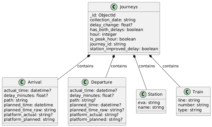
MongoDB document schema: Journeys collection containing nested Arrival, Departure, Station, and Train subdocuments

Transformed document schema: each journey links planned timetable data with real-time delays via journey_id matching

Technical Decisions

MongoDB over a relational database: The DB API returns deeply nested XML with variable schemas — trains may have arrivals only, departures only, or both, and change records include optional fields like platform changes and cancellation flags. MongoDB’s flexible schema handles this naturally without requiring upfront DDL or null-heavy relational tables. The aggregation framework also maps well to the analytical transformations needed.

ELT over ETL: Loading raw API responses before transforming preserves the original data for replay and debugging. When I discovered the API only retains ~12 hours of historical data (undocumented), I had to redesign the collection strategy from bulk historical pulls to multiple daily runs at strategic times (22:00). Having raw data already loaded meant I didn’t lose earlier collections during this pivot.

Compound unique indexing (station_eva + date + hour): The collection functions run on overlapping schedules to maximize coverage. Without deduplication at the database level, repeated runs would inflate counts. The compound index prevents this silently via upsert, so the pipeline is idempotent — critical for a system designed to run repeatedly.

Key Findings

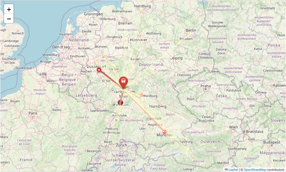
Folium map showing Frankfurt Hbf's connections radiating to destinations across Germany, Austria, Switzerland, and the Netherlands

Frankfurt Hbf: 203 unique destinations — connections extend into Austria, Switzerland, the Netherlands, and Belgium

Hub size does not predict operational efficiency. Mannheim Hbf, a mid-tier hub, achieves the best delay recovery (-1.0 min average delay_change, 40.3% recovery rate), while larger hubs like Frankfurt (+0.7 min) and Hamburg (+0.3 min) actually add delays on average. The worst performer, Erfurt Hbf (+1.3 min, 20.8% recovery), suggests that factors like scheduled turnaround buffers, platform utilization, and traffic composition matter more than infrastructure investment alone.

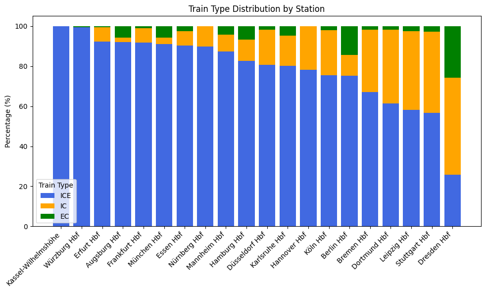
Stacked bar chart showing ICE/IC/EC distribution across 20 stations — Kassel-Wilhelmshoehe at 100% ICE, Dresden at only 25%

Train type specialization: major hubs show 90%+ ICE dominance, while regional stations like Dresden have more balanced IC/EC mixes

The network is hub-dependent and hierarchical. Frankfurt (203 connections), Munich (187), and Stuttgart (186) dominate connectivity. These same hubs show >90% ICE specialization, confirming their role as long-distance consolidation points — yet as RQ1 showed, these high-connectivity hubs don’t necessarily manage delays efficiently.

Horizontal bar chart of top 20 rail corridors — Berlin to Berlin Ostbahnhof leads with 343 trains, followed by Nuernberg to Munich at 300

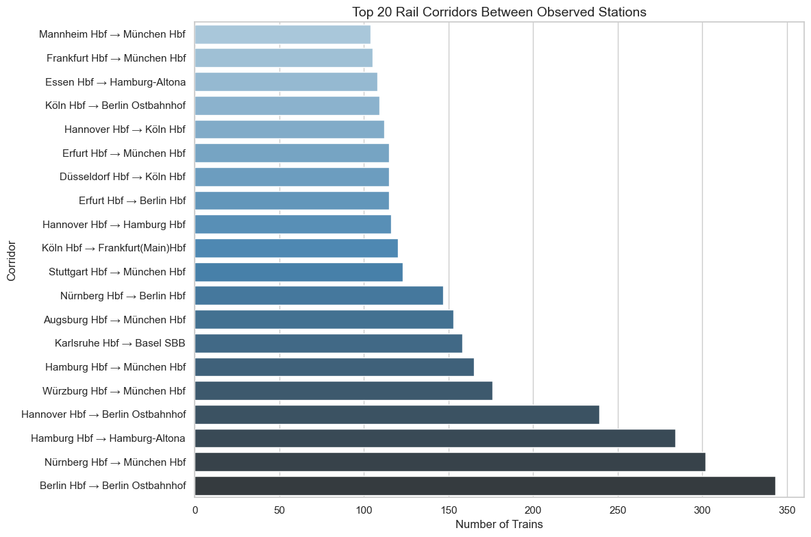
Top 20 corridors: short-distance terminal flows (Berlin→Ostbahnhof) reflect end-of-line journey legs, not standalone trips

Corridor analysis reveals two distinct network patterns. Balanced bidirectional trunk lines (Karlsruhe–Leipzig: imbalance ratio 0.0) form the operational backbone, while completely asymmetric terminal flows (Berlin Hbf→Berlin Ostbahnhof: 343 trains, all one direction) represent end-of-line journey legs. This distinction is important for capacity planning — balanced corridors need symmetric infrastructure, while terminal segments face directional congestion.

Evening peak delays cascade into late night. Average delays reach 17.2 minutes by 19:00 and persist at 20.9 minutes at 21:00 despite sharply declining train volumes. This counterintuitive pattern — fewer trains but higher delays — indicates that congestion-induced disruptions during peak hours create operational debts that propagate through the remaining schedule.

What I Learned

The most valuable engineering lesson came from the API itself. The DB documentation doesn’t mention that historical data is only retained for ~12 hours. I discovered this after my initial plan to pull a full week in bulk failed silently — the API returned empty responses for older time windows without error codes. This forced a complete redesign from batch historical collection to scheduled daily runs, and reinforced that early API exploration and boundary testing should happen before committing to an architecture.

The second insight was about debugging data pipelines specifically: errors manifest as silent data quality issues rather than runtime exceptions. A single-character typo in a field name within a MongoDB aggregation pipeline took hours to trace because the pipeline ran successfully — it just produced wrong numbers. This highlighted the importance of validation at data boundaries, not just code boundaries.

Limitations

The analysis covers 6 days of data (Oct 15–21, 2025) — sufficient to demonstrate the pipeline and identify structural patterns, but not enough for seasonal analysis or statistical robustness. With more time, I’d extend collection over several months and incorporate weather data as a covariate.

Technology Stack

Database: MongoDB Atlas (pymongo, compound indexing, aggregation pipelines with $lookup, $unwind, $group, $addToSet)
Data Acquisition: Deutsche Bahn OpenData API, XML parsing (ElementTree), rate-limited collection orchestration
Analysis: Python, pandas, matplotlib, seaborn
Geo-visualization: Folium (interactive maps with OpenStreetMap + Nominatim geocoding)

Read the full 65-page report (PDF) — covers the complete ELT implementation, all five research questions with code, and detailed analysis.